SNNS (of JavaNNS) is a tool that permits you to build, train, and
evaluate different types of Neural Networks. For this assignment you
are going to build a standard backpropagation Neural Network with
sigmoid units. The output units can be chosen to be either sigmoid or
linear units (which would permit an output larger than 1.0.
In
SNNS (or JavaNNS) you can build your network graphically on the
screen using the bignet tool. It permits you to specify the units per
layer, their type, and the connectivity. The easiest is simply to
fully connect the successive layers.
To train the network you
have to create a file with the training data and load it into the
training window. Select random initialization and reshuffeling of the
patterns. The learning function should be standard backpropagation.
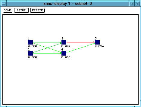
First create a netrwork. For XOR, a network with 2 input units, two hidden units and one output unit is sufficient. Since the desired output is always 0 or 1 we can use a sigmoid unit as output unit, too. To create the network go to Bignet and create a new feedforward network. Create a first layer with 2 (1x2) input units, create a second layer with 2 (1x2) hidden units, and create a third layer with 1 output unit. Then select fully connect to connect all the units of each layer to all the units of the next layer. Select create network and quit Bignet. If you select Display it will show you the network (you have to tell it under setup that you want the links to be displayed).

To train the network you first have to generate a file with training instances. The file has to have the following format (# indicates a comment):
SNNS pattern definition file V3.2
generated at Mon Apr 25 15:58:23 1994

No. of patterns : 4
No. of input units : 2
No. of output units : 1

# Input pattern 1:
0 0
# Output pattern 1:
0
# Input pattern 2:
0 1
# Output pattern 2:
1
# Input pattern 3:
1 0
# Output pattern 3:
1
# Input pattern 4:
1 1
# Output pattern 4:
0
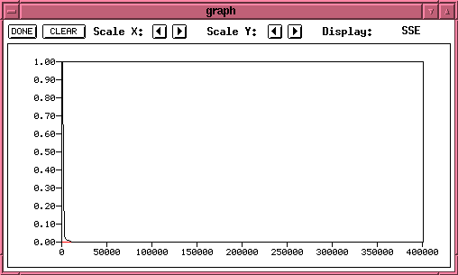
Load the pattern file into the simulator, open the graph window to see the learning curve and then go to Control (the training functions). Select standard backpropagation as the learning rule and randomized weights as the initialization method. Then select shuffle in the cycles row (this is where you train all the patterns and shuffle indicates that the order is changed every cycle). Set the number of cycles to 10000, press init (in the steps row) to initialize the weights, and then press all in the cycles row to train the network for 10000 cycles. You should see a curve appear in the graph window which shows a decreasing error reaching approximately 0 after a few thousand cycles.

Don't forget to save your network before you leave the simulator!
Jahmm is a java library that provides functionality for learning
and use of Hidden Markov Models. To learn a HMM you have to specify
its size (i.e. How many states and how many different observations
are there).
To train the HMM you have to put the training data
(in this case multiple sequences of observations) into the
appropriate vector structure. Discrete observations here are
represented as integers and the observations structure is a vector of
vectors, each of which represents a sequence of ObservationInteger
objects. Learning itself is achieved using one of two algorithms,
K-means approximation and Baum-Welch. The latter is a local
optimization algorithm and therefore needs an initial HMM. The
easiest way is to let K-means generate the initial HMM and then use
Baum-Welch to optimize the initial HMM.
Once a HMM is learned the
jahmm package permits to save the HMM as a .dot file (which can be
converted to a graphical representation using the dot program (part
of the freely available graphViz package).
To make predictions
using the learned HMM, you have to first find the state with the
highest probability of being the one the system is in right now. This
is done using the Viterbi algorithm which identifies the most likely
state sequence to have generated the given sequence of observations.
Given this state you can calculate the most likely next observation.
Assume that there are coins, one being biased towards heads (60% of the time it lands heads), one biased towards tails (60% of the time it lands tails). Assume further that a person picks up one of the coins and starts flipping it repeatedly (without you knowing which coin it is). From the sequence of results (heads or tails), learn a model that predicts if the next observation will be heads or tails. To do this (actually without knowing that the coins are biased or how biased they are) we can set up a HMM learner that learns a HMM that models the process of flipping the coin. In this case we decide to let it learn a HMM with 2 states and 2 observations (heads =0, tails = 1). Two states should be sufficient there are only two possible coins.
The following program shows how to learn a HMM for this problem. The data array in the beginning contains 42 sequences of 100 coin flips each (each sequence represents a new trial, i.e. It might be using either of the two coins).
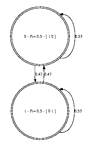
You can compile this program using javac -classpath .:jahmm-0.2.2.jar HmmExample_coin.java (assuming the jahmm library is in the current directory) and run it using java -classpath .:jahmm-0.2.2.jar HmmExample_coin . The program learns a HMM by first training it using the K-means algorithm and then running 11 iternations of the Baum-Welch algorithms. The following shows the resulting HMM plotted using the dot program:

This
shows that the HMM learner learned a HMM where each state represents
one of the faces of the coin (heads or tails). Furthermore the
probability of heads if in the heads state is 0.53 while the one for
tails is 0.47. This shows that the HMM did not completely learn the
correct model but identified some of the important aspects.
hmm contains a number of executables to learn and evaluate Hidden Markov Models. In particular, it contains a routine to train (and optimize) an initial HMM using Baum-Welch and a program to determine the most likely sequence of states corresponding to a given observation sequence using the Viterbi algorithm.
To learn a HMM you have to specify an initial model in the files
modelname.trans and modelname.emit. modelname.trans
contains the transition probabilities between states in the
initial model in the form "fromstate tostate probability".
You can give the states in your HMM arbitrary names with the
exception of INIT which is a special state that the system
starts from. Transition probabilities from state INIT to any
of your states represent the probabilities that the system starts in
the given state. modelname.emit contains the probabilities
with which any given state is tied to a particular observation in the
form "state observation probability". When
generating an initial model, be careful not to incorrectly assign too
many probabilities that are equal to 0 since this might make it
impossible for your model to generate the data sequence. This would
lead to an error since the result of the evaluation of the Baum-Welch
algorithm would return 0. To train the HMM you have to put the
training data (in this case multiple sequences of observations) into
the file modelname.train. You can then train the HMM by
calling "src/trainhmm modelname resultmodelname
modelname.train". This runs the Baum-Welch algorithm over
your model and generates the final optimized model in the files
resultmodelname.trans and resultmodelname.emit .
To
make predictions using the learned HMM, you have to first find the
state with the highest probability of being the one the system is in
right now. This is done using the Viterbi algorithm which identifies
the most likely state sequence to have generated the given sequence
of observations. Given this state you can calculate the most likely
next observation.
Assume that there are two coins, one being biased towards heads (60% of the time it lands heads), one biased towards tails (60% of the time it lands tails). Assume further that a person picks up one of the coins and starts flipping it repeatedly (without you knowing which coin it is). From the sequence of results (heads or tails), learn a model that predicts if the next observation will be heads or tails. To do this (actually without knowing that the coins are biased or how biased they are) we can set up a HMM learner that learns a HMM that models the process of flipping the coin. In this case we decide to let it learn a HMM with 2 states and 2 observations (heads =C1, tails = C2). Two states should be sufficient there are only two possible coins.
The following files show an initial model for this problem. The training data contains 42 sequences of 100 coin flips each (each sequence represents a new trial, i.e. It might be using either of the two coins).
You can now train the HMM using the trainhmm executable which will run approximately 5 iterations of Baum-Welch until it converges. The resulting HMM represents a system where each state represents one of the faces of the coin (heads or tails). Furthermore the probability of heads if in the heads state is 0.53 while the one for tails is 0.48. This shows that the HMM did not completely learn the correct model but identified some of the important aspects.